Background
How many groups, or types, of Star Wars characters are there? I’ve been wanting to use the starwars dataset built-in to the dplyr package, and at the same time, have been working hard on an R package to carry out an analysis suited to doing this. Part of the challenge of using the approach in this R package is determining how groups groups there are.
Many approaches (Latent Profile Analysis, for example) use Maximum Likelihood estimation (while the approach I’ve developed uses a two-step cluster analysis based around the geometric (and algebraic) idea of “distance”, or how close (similar) observations are). This is easy enough when we’re talking about something like length. If something is 4 long and another thing 8, then what is there distance (4!)? When we’re talking about more than just length - say, length and width - then it’s the exact same idea, except the distance represents how far two things are across both measures - length and width.
But back to groups of Star Wars characters. How many are there? Let’s see what data we have:
library(dplyr)

starwars
## # A tibble: 87 x 13
## name height mass hair_color skin_color eye_color birth_year gender
## <chr> <int> <dbl> <chr> <chr> <chr> <dbl> <chr>
## 1 Luke… 172 77 blond fair blue 19 male
## 2 C-3PO 167 75 <NA> gold yellow 112 <NA>
## 3 R2-D2 96 32 <NA> white, bl… red 33 <NA>
## 4 Dart… 202 136 none white yellow 41.9 male
## 5 Leia… 150 49 brown light brown 19 female
## 6 Owen… 178 120 brown, gr… light blue 52 male
## 7 Beru… 165 75 brown light blue 47 female
## 8 R5-D4 97 32 <NA> white, red red NA <NA>
## 9 Bigg… 183 84 black light brown 24 male
## 10 Obi-… 182 77 auburn, w… fair blue-gray 57 male
## # … with 77 more rows, and 5 more variables: homeworld <chr>, species <chr>,
## # films <list>, vehicles <list>, starships <list>It looks like we only have three measures that are numbers (height, mass, and birth_year) - though there are others we could possibly turn into numbers (maybe), and there are other approaches (Latent Class Analysis) that can deal with non-numeric measures (such as hair_color). But we’ll have to stick to the three measures that are numbers, for better or worse, for now.
R2
Let’s first take a look at the plot of R2 values, which are obtained from the second of the two steps of the cluster analysis - the k-means step (I say this because there are other, perhaps better, ways to calculate the R-squared values, such as from a MANOVA).
We just list the name of the data and the variables we would like to use. Since birth_year is on a very different metric than the other two variables, we’ll set to_scale and to_center to TRUE. We’ll also return a table, instead of a plot.
library(prcr)

plot_r_squared(starwars, height, mass, birth_year, to_scale = TRUE, to_center = TRUE, r_squared_table = T)
## ################################## Clustering data for iteration 2## Clustering data for iteration 3## Clustering data for iteration 4## Clustering data for iteration 5## Clustering data for iteration 6## Clustering data for iteration 7## Clustering data for iteration 8## Clustering data for iteration 9## ################################## cluster r_squared_value
## 1 2 0.507
## 2 3 NA
## 3 4 NA
## 4 5 NA
## 5 6 NA
## 6 7 NA
## 7 8 NA
## 8 9 NAOoh! Not good. Before the second of the two steps settled on the groups, it ended up with a group with no observations. This is probably in part the result of a small sample, and possibly attributable to the measures we used - and maybe some missing data for some of the measures. Let’s take a look at the data:
starwars_ss <- select(starwars, height, mass, birth_year)
skimr::skim(starwars_ss)| Name | starwars_ss |
| Number of rows | 87 |
| Number of columns | 3 |
| _______________________ | |
| Column type frequency: | |
| numeric | 3 |
| ________________________ | |
| Group variables | None |
Variable type: numeric
| skim_variable | n_missing | complete_rate | mean | sd | p0 | p25 | p50 | p75 | p100 | hist |
|---|---|---|---|---|---|---|---|---|---|---|
| height | 6 | 0.93 | 174.36 | 34.77 | 66 | 167.0 | 180 | 191.0 | 264 | ▁▁▇▅▁ |
| mass | 28 | 0.68 | 97.31 | 169.46 | 15 | 55.6 | 79 | 84.5 | 1358 | ▇▁▁▁▁ |
| birth_year | 44 | 0.49 | 87.57 | 154.69 | 8 | 35.0 | 52 | 72.0 | 896 | ▇▁▁▁▁ |
It looks like the birth_year is missing for a lot - 44 - of the observations for the 87 Star Wars characters we have. We’re down to the bare-bones number of measures, but let’s try with just height and mass. We probably don’t need to scale the data.
plot_r_squared(starwars, height, mass, to_scale = TRUE, to_center = TRUE, r_squared_table = T)## ################################## Clustering data for iteration 2## Clustering data for iteration 3## Clustering data for iteration 4## Clustering data for iteration 5## Clustering data for iteration 6## Clustering data for iteration 7## Clustering data for iteration 8## Clustering data for iteration 9## ################################## cluster r_squared_value
## 1 2 0.485
## 2 3 0.872
## 3 4 NA
## 4 5 NA
## 5 6 0.977
## 6 7 NA
## 7 8 NA
## 8 9 NAThat’s better - in a sense. We have two, three, and six groups solutions. I wouldn’t trust the six group solution very much. The R2 value does increase substantialy between two and three groups. This suggests maybe there are three groups (when we use just the measures for weight and mass).
Groups
two_profiles <- create_profiles(starwars, height, mass, n_profiles = 2, to_scale = TRUE, to_center = TRUE)
plot(two_profiles)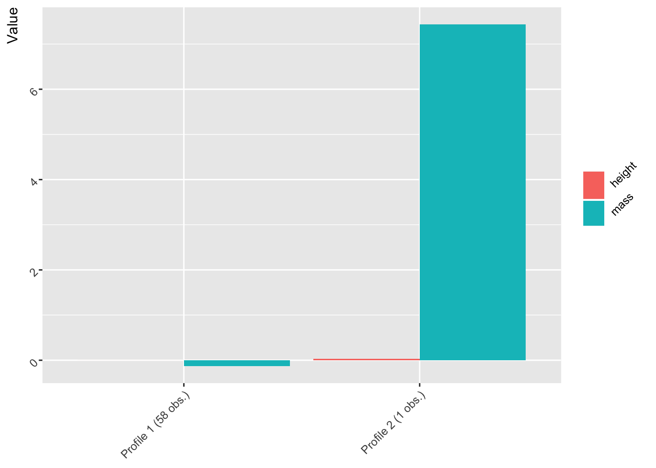
three_profiles <- create_profiles(starwars, height, mass, n_profiles = 3, to_scale = TRUE, to_center = TRUE)
plot(three_profiles)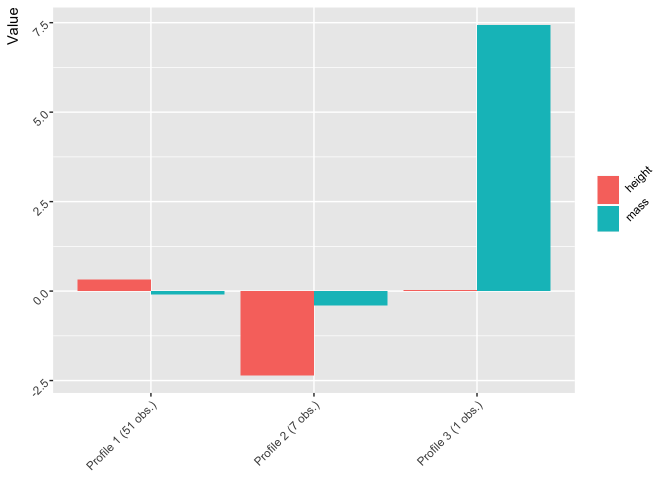
The third group: Massive, not so tall
It looks like there is one very massive (literally) observation that makes up one profile in both the two and three profile solutions. Who is it?
three_profiles$.data %>%
    filter(cluster == 3) %>%
knitr::kable()| name | height | mass | hair_color | skin_color | eye_color | birth_year | gender | homeworld | species | films | vehicles | starships | cluster |
|---|---|---|---|---|---|---|---|---|---|---|---|---|---|
| Jabba Desilijic Tiure | 175 | 1358 | NA | green-tan, brown | orange | 600 | hermaphrodite | Nal Hutta | Hutt | c(“The Phantom Menace”, “Return of the Jedi”, “A New Hope”) | character(0) | character(0) | 3 |
Jabba. Of course. It looks like with two or three groups, Jabba ends up in one cluster.
The second group: Less massive, small height
What about the seven - who seem to be less massive and with a small height - in the second group?
three_profiles$.data %>%
    filter(cluster == 2) %>%
knitr::kable()| name | height | mass | hair_color | skin_color | eye_color | birth_year | gender | homeworld | species | films | vehicles | starships | cluster |
|---|---|---|---|---|---|---|---|---|---|---|---|---|---|
| R2-D2 | 96 | 32 | NA | white, blue | red | 33 | NA | Naboo | Droid | c(“Attack of the Clones”, “The Phantom Menace”, “Revenge of the Sith”, “Return of the Jedi”, “The Empire Strikes Back”, “A New Hope”, “The Force Awakens”) | character(0) | character(0) | 2 |
| R5-D4 | 97 | 32 | NA | white, red | red | NA | NA | Tatooine | Droid | A New Hope | character(0) | character(0) | 2 |
| Yoda | 66 | 17 | white | green | brown | 896 | male | NA | Yoda’s species | c(“Attack of the Clones”, “The Phantom Menace”, “Revenge of the Sith”, “Return of the Jedi”, “The Empire Strikes Back”) | character(0) | character(0) | 2 |
| Wicket Systri Warrick | 88 | 20 | brown | brown | brown | 8 | male | Endor | Ewok | Return of the Jedi | character(0) | character(0) | 2 |
| Sebulba | 112 | 40 | none | grey, red | orange | NA | male | Malastare | Dug | The Phantom Menace | character(0) | character(0) | 2 |
| Dud Bolt | 94 | 45 | none | blue, grey | yellow | NA | male | Vulpter | Vulptereen | The Phantom Menace | character(0) | character(0) | 2 |
| Ratts Tyerell | 79 | 15 | none | grey, blue | unknown | NA | male | Aleen Minor | Aleena | The Phantom Menace | character(0) | character(0) | 2 |
These seem to be droids, Yoda, and some other tiny characters.
(Some from) the first group: Above average height, below average mass
The 51 in the first group, with slightly above average height, and slightly below average mass? It’s a big group, so here are just the first six, with a lot of familiar characters:
three_profiles$.data %>%
    filter(cluster == 1) %>%
    head() %>%
knitr::kable()| name | height | mass | hair_color | skin_color | eye_color | birth_year | gender | homeworld | species | films | vehicles | starships | cluster |
|---|---|---|---|---|---|---|---|---|---|---|---|---|---|
| Luke Skywalker | 172 | 77 | blond | fair | blue | 19.0 | male | Tatooine | Human | c(“Revenge of the Sith”, “Return of the Jedi”, “The Empire Strikes Back”, “A New Hope”, “The Force Awakens”) | c(“Snowspeeder”, “Imperial Speeder Bike”) | c(“X-wing”, “Imperial shuttle”) | 1 |
| C-3PO | 167 | 75 | NA | gold | yellow | 112.0 | NA | Tatooine | Droid | c(“Attack of the Clones”, “The Phantom Menace”, “Revenge of the Sith”, “Return of the Jedi”, “The Empire Strikes Back”, “A New Hope”) | character(0) | character(0) | 1 |
| Darth Vader | 202 | 136 | none | white | yellow | 41.9 | male | Tatooine | Human | c(“Revenge of the Sith”, “Return of the Jedi”, “The Empire Strikes Back”, “A New Hope”) | character(0) | TIE Advanced x1 | 1 |
| Leia Organa | 150 | 49 | brown | light | brown | 19.0 | female | Alderaan | Human | c(“Revenge of the Sith”, “Return of the Jedi”, “The Empire Strikes Back”, “A New Hope”, “The Force Awakens”) | Imperial Speeder Bike | character(0) | 1 |
| Owen Lars | 178 | 120 | brown, grey | light | blue | 52.0 | male | Tatooine | Human | c(“Attack of the Clones”, “Revenge of the Sith”, “A New Hope”) | character(0) | character(0) | 1 |
| Beru Whitesun lars | 165 | 75 | brown | light | blue | 47.0 | female | Tatooine | Human | c(“Attack of the Clones”, “Revenge of the Sith”, “A New Hope”) | character(0) | character(0) | 1 |
Cross-validation
The other technique for determining the number of groups, cross-validation, may be folly because of how it works: Split the data into two, and see how well groups in one half can be reproduced in the other. This may be a problem due to the Jabba-group.
We’ll use the same arguments except for plot_r_squared, which we don’t need, and for one argument, n_profiles, for how many groups we want to cross-validate the groupings for (we have to deal with complete cases, which is what the first two lines are for), for the three group solution:
starwars_ss <- starwars_ss[complete.cases(starwars_ss), ]
cross_validate(starwars_ss, height, mass, n_profiles = 2, to_scale = TRUE, to_center = TRUE)
Not pretty. Convergence issues galore (I decided not to print the messages because there were so many). The Fleiss’ Kappa was close to 0; the percentage agreement 0.61.
Conclusion
Looking at height and weight, we seem to be able to identify three broad groups of Star Wars characters. However, we shouldn’t have a ton of confidence in howe well these groups generalize to all Star Wars characters: Our sample is small, the measures we could use were limited, and our cross-validation did not provide us with much evidence to back up our three distinct groups.
On the other hand, we did have a starting point for how many groups to look for from our R2 values, which was good, and the groups seem interpretable on the basis of those characters in our three groups.
Try it out
The prcr package used to create the groups and calculate the R2 values is available in R using install.packages("prcr"). An in-development version with the function for cross-validation is available using the following two commands (if you have devtools installed already then only the second command is needed:
install.packages("devtools")
devtools::install_github("jrosen48/prcr")
Thanks and credit to Rebecca Steingut now at Teachers’s College - Columbia University for contributing to the in-development version of the package and the cross validation strategy implemented in it.