Note - an R package for carrying out Latent Profile Analysis (LPA): tidyLPA
Since writing this post, I have worked with colleagues to release an R package to carry out the analysis. The package is tidyLPA and is described in the following sections, through the “Original Post” header below which is the beginning of the original post.
Introduction
Latent Profile Analysis (LPA) is a statistical modeling approach for estimating distinct profiles, or groups, of variables. In the social sciences and in educational research, these profiles could represent, for example, how different youth experience dimensions of being engaged (i.e., cognitively, behaviorally, and affectively) at the same time.
tidyLPA provides the functionality to carry out LPA. LPA is a statistical modeling approach for estimating parameters (i.e., the means, variances, and covariances) for profiles. Note that tidyLPA is still at the beta stage! Please report any bugs at https://github.com/jrosen48/tidyLPA or send an email to jrosen@msu.edu.
Installation
You can install tidyLPA from CRAN with:
install.packages("tidyLPA")You can also install the in-development version of tidyLPA from GitHub with:
install.packages("devtools")
devtools::install_github("jrosen48/tidyLPA")
Example
Here is a brief example using the built-in pisaUSA15 dataset and variables for broad interest, enjoyment, and self-efficacy. Note that we first type the name of the data frame, followed by the unquoted names of the variables used to create the profiles. We also specify the number of profiles and the model. See ?estimate_profiles for more details.
library(tidyLPA)## Note that an update to tidyLPA is forthcoming; see vignette('introduction-to-major-changes') for details!d <- pisaUSA15[1:100, ]
m3 <- estimate_profiles(d,
broad_interest, enjoyment, self_efficacy,
n_profiles = 3)## Fit Equal variances and covariances fixed to 0 (model 1) model with 3 profiles.## LogLik is 283.991## BIC is 631.589## Entropy is 0.914plot_profiles(m3, to_center = TRUE)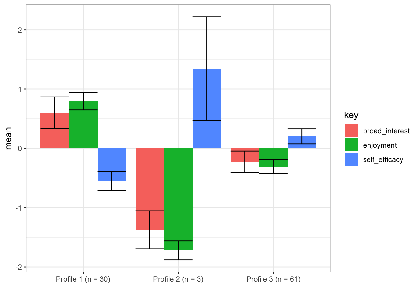
Learn more
To learn more:
Contact
As tidyLPA is at an early stage of its development, issues should be expected. If you have any questions or feedback, please do not hesitate to get in touch:
- By email (jrosen@msu.edu)
- By Twitter
- Through filing an issue on GitHub here
Please note that this project is released with a Contributor Code of Conduct. By participating in this project you agree to abide by its terms.
Original Post
Background
Along with starting to use MPlus, I’ve become (more) interested in trying to find out how to carry out Latent Profile Analysis (LPA) in R, focused on two options: OpenMx and MCLUST. The two are very different: OpenMx is an option for general latent variable modeling (i.e., it can be used to specify a wide range of latent variable models, from Confirmatory Factor Analysis to a Growth Mixture Model), while MCLUST is (primarily) for clustering (and classification) using mixture models.This post is a first attempt about carrying out LPA using MCLUST in R. MCLUST does model-based clustering, as or as the authors describe it, Gaussian Mixture Modeling, since LPA can be seen as one way to do mixture modeling through general latent variable modeling software. Another post will focus on OpenMx (and MPlus), both of which do that.
LPA models
When carrying out LPA, we can fit an unconstrained model, in which not only the measured variables’ means, but also their variance and covariances, are different, or freely-estimated, across profiles, or mixture components. However, we also sometimes estimate commonly-specified models that are more constrained as part of a model-building process.
Namely, we are commonly interested in those in which the residual variances are constrained (to be the same across components) or freely-estimated (to be different across components) and the covariances are fixed (to be zero, i.e. the covariance matrix is diagonal, in that only the cells on the diagonal, or the variances, are estimated) or freely-estimated.
Let’s get started.
Test (example) code using the “iris” data
Here is a first pass, using the iris data, which is built into R.
First, let’s explore fit indices for each of the three models with between one and six mixture components. Like MCLUST does in its built-in function, we can plot these values of the Bayesian Information Criteria (BIC).
library(tidyverse, warn.conflicts = FALSE)
library(mclust)
library(hrbrthemes)

data(iris)

df <- select(iris, -Species)

explore_model_fit <- function(df, n_profiles_range = 1:9, model_names = c("EII", "VVI", "EEE", "VVV")) {
    x <- mclustBIC(df, G = n_profiles_range, modelNames = model_names)
    y <- x %>%
        as.data.frame.matrix() %>%
        rownames_to_column("n_profiles") %>%
        rename(`Constrained variance, fixed covariance` = EII,
               `Freed variance, fixed covariance` = VVI,
               `Constrained variance, constrained covariance` = EEE,
               `Freed variance, freed covariance` = VVV)
    y
}

fit_output <- explore_model_fit(df, n_profiles_range = 1:6)

to_plot <- fit_output %>%
    gather(`Covariance matrix structure`, val, -n_profiles) %>%
    mutate(`Covariance matrix structure` = as.factor(`Covariance matrix structure`),
           val = abs(val)) # this is to make the BIC values positive (to align with more common formula / interpretation of BIC)

library(forcats)

to_plot$`Covariance matrix structure` <- fct_relevel(to_plot$`Covariance matrix structure`,
                                                     "Constrained variance, fixed covariance",
                                                     "Freed variance, fixed covariance",
                                                     "Constrained variance, constrained covariance",
                                                     "Freed variance, freed covariance")


ggplot(to_plot, aes(x = n_profiles, y = val, color = `Covariance matrix structure`, group = `Covariance matrix structure`)) +
    geom_line() +
    geom_point() +
    ylab("BIC (smaller value is better)") +
    theme_ipsum_rc()
From red to purple, the models become less constrained (more free). It appears that a two or three profile (mixture component) model with freely-estimated residual variances and covariances, or a four profile model with constrained residual covariances and variances, fit best (based on interpreting the BIC).
Given this, we can fit (and inspect) a model, say, the three profile model with freely-estimated residual variance and covariances.
create_profiles_mclust <- function(df,
                                   n_profiles,
                                   variance_structure = "freed",
                                   covariance_structure = "freed"){

    if (variance_structure == "constrained" & covariance_structure == "fixed") {

        model_name <- "EEI"

    } else if (variance_structure == "freed" & covariance_structure == "fixed") {

        model_name <- "VVI"

    } else if (variance_structure == "constrained" & covariance_structure == "constrained") {

        model_name <- "EEE"

    } else if (variance_structure == "freed" & covariance_structure == "freed") {

        model_name <- "VVV"

    } else if (variance_structure == "fixed") {

        stop("variance_structure cannot equal 'fixed' using this function; change this to 'constrained' or 'freed' or try one of the models from mclust::Mclust()")

    }

    x <- Mclust(df, G = n_profiles, modelNames = model_name)

    print(summary(x))

    dff <- bind_cols(df, classification = x$classification)

    proc_df <- dff %>%
        mutate_at(vars(-classification), scale) %>%
        group_by(classification) %>%
        summarize_all(funs(mean)) %>%
        mutate(classification = paste0("Profile ", 1:n_profiles)) %>%
        mutate_at(vars(-classification), function(x) round(x, 3)) %>%
        rename(profile = classification)

    return(proc_df)

}

m3 <- create_profiles_mclust(df, 3, variance_structure = "freed", covariance_structure = "freed")
We can then plot the mean values for the variables used to estimate the model for each of the two profiles. Of course, there are other models that we may want to inspect with different covariance matrix structures or profile numbers.
m3 %>%
    gather(key, val, -profile) %>%
    ggplot(aes(x = profile, y = val, fill = key, group = key)) +
    geom_col(position = "dodge") +
    ylab("Z-score") +
    xlab("") +
    scale_fill_discrete("") +
    theme_ipsum_rc()
Please send me a message if you have any comments.
A big thank you to my colleagues You-Kyung Lee and Kristy Robinson for helping me begin to understand LPA.